Lossless Data Compression of AIRS Signals (Overview)
 We have made an attempt to design a lossless compression algorithm
specifically tailored for the sounder data. The algorithm
(applied on digital counts) consists of the following steps:
We have made an attempt to design a lossless compression algorithm
specifically tailored for the sounder data. The algorithm
(applied on digital counts) consists of the following steps:
- Step 1: Channel Partitioning
- Step 2: Whitening
- Reduction of oscillatory pattern
- adaptive clustering
- Step 3: Projection (dimensionality reduction)
- Step 4: Estimated entropy coding
- Reduction of oscillatory pattern
- adaptive clustering
The stages of the algorithm can be visualized via the diagram 1.
In what follows, we give a brief description of each step of the algorithm.
Step 1: Channel Partitioning
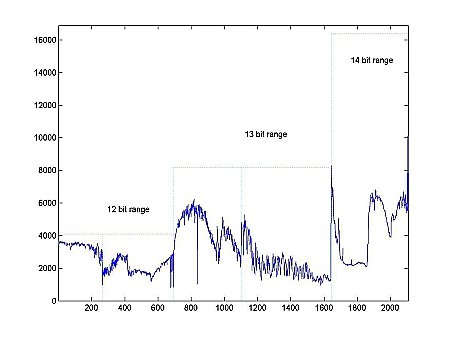
During the first stage, the original $90 \times 135 \times 2107$ granule is subdivided into 5 bands of size Kn, so that Σ5 Kn = 2107. This maximizes the continuity of each unit and takes into account that the range of the digital counts varies (12, 13, and 14 bits) with channel index. After this subdivision, each of the resulting 90 x 135 x Kn granules will be processed (steps 2 through 4 of the diagram) independently.
Step 2: Whitening
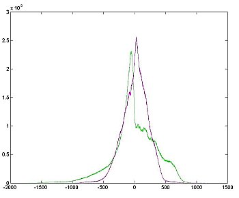
The purpose of the whitening stages is to transform the data so that its distribution is as close to normal as possible. The cost of this transformation is added memory utilization (due primarily to record-keeping data structures needed for the decompression procedure). There are several theorems which state an optimality (in some sense) of the Karhunen-Loeve transform provided a normal distribution of the data. Therefore, if the whitening stage is "cheap" in terms of memory utilization, overall transformation (steps 1-4) is nearly optimal. We have two consecutive steps (labeled (a) and (b) on the diagram) to achieve this effect. The amount of space needed for step 2 is 12*(K_1+K_2) + 13(K_3+K_4) + 14*K_5 = &Sigma5 bn Kn, where bn is the number of bits needed to store the oscillatory component in each of the five bands, and for step 3 is $\sum^{5}_{n=1} L_n b_n K_n + I J \sum^5_{n=1} \log_2(L_n)$, where $L_n$ is the number of clusters used. The ratio of memory needed for steps 1-3 with respect to the total memory occupied by the original granule varied in the 10 considered granules, but on average was approximately 1288:1, i.e. about $ 0.037 \%$ of the memory used by original granule is needed to force the data to have almost normal distribution. We felt that this was a relatively low cost for a known optimal approach and so have proceeded along that course.
 |
 |
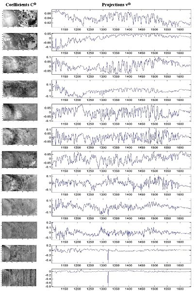
Step 3: Dimensionality Reduction
As alluded to in the previous section, we apply the Karhunen-Loeve transform and it is known to have the smallest average error when approximating a class of functions by their projection on $L$ orthogonal vectors chosen a priori. If the goal was to develop a lossy algorithm, our primary cost would be the error and we would have to define a notion of acceptable average error to determine the number $L$ of projection vectors. Since we design a lossless compression algorithm, our primary cost is memory utilization and we need to define a notion of minimal memory space to save both projection vector coefficients and the residuals of the projection. The number $L_n$ of the projection vectors is chosen to address this concern. Thus, during the dimensionality reduction (stage 4 of the diagram) the global part of the information from each of the 5 bins is saved in $L$ packets, where each packet contains a $90 \times 135$ image of the coefficients $C_l$ and a $1 \times K_n$ projection vectors $v_l$, resulting in $L (90 \cdot 135 + K_n)$ elements in total. The reconstruction formula $\tilde{a}_{i j k}=\sum_{l=1}^{L_n} C_l \cdot v_l $ is used to compute an approximation $\tilde{a}_{ijk}$ for each element $a_{ijk}$. The differences $r_{ijk}=a_{ijk} - \tilde{a}_{ijk}$, called residuals, are saved separately through the last (approximated entropy coding) stage of our lossless compression algorithm.
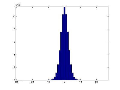
Step 4: Approximated Entropy Coding
After step 3, we have $90 \times 135 \times K_n$ granules of residuals that are approximately normally distributed but have a lower entropy (due to properties of Karhunen-Loeve transform). In our computations, the entropy on the average decreased from 10.35 to 3.5 during step 3. Therefore, the lower bound on the number of bits per residual entry $r_{ijk}$ is 3.5 bits. We build our Huffman codebook based on a normal distribution with variance computed from the residuals, rather than an actual codebook. This mitigates issues with errors during transmission, and also makes our program slightly more efficient.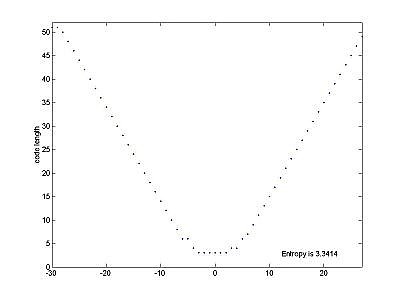 |
 |
Results
| Granule | Location | Ratio |
|---|---|---|
| 9 | Pacific Ocean, Daytime | 3.2424 |
| 16 | Europe, Nighttime | 3.2495 |
| 60 | Asia, Daytime | 3.1893 |
| 82 | North America, Nighttime | 3.2750 |
| 120 | Antarctica, Nighttime | 3.1947 |
| 126 | Africa, Daytime | 3.1769 |
| 129 | Arctic, Daytime | 3.2848 |
| 151 | Australia, Nighttime | 3.1367 |
| 182 | Asia, Nighttime | 3.0851 |
| 193 | North America, Daytime | 3.1563 |
Ongoing Work
- Adaptive Partitioning: The choice of partitions has substantial effect on the compression ratio, so more work needs to be done on implementation and certification of algorithms for choosing optimal partitions.
- Entropy Coding: The current version of the algorithm only entropy codes the residuals, and does not do anything to the coefficients themselves. The images' structure indicates that compression is possible on the coefficient images as well.
- Assembly Programming: The software will reside onboard the real-time satellite system, and, therefore, must be optimized to operate in this environment. The upper bound on the entire procedure is 12 seconds during which time it must process 1 granule (6 minutes or 231.1416 MB of data). For the new GOES-R system, the data rate is 34 times greater. Therefore, some assembly will be written along key execution paths (especially in the advanced mathematical subroutines -- eigenvector calculation, etc).